Particles can be sampled for unbiased estimates of volume in a number weighted, volume weighted, or surface-weighted manner. For number weighted estimates thick sections are used since a disector is required. For volume weighted and surface weighted estimated thin sections can be used. The probes that are used to estimate the volume of particles are the nucleator, the planar rotator, the optical rotator, point-sampled-intercepts, and surface weighted star volume. The discrete vertical rotator has been developed for estimating the volume of organelles at the electron microscope level. Traditionally, due to ease of use and continuity, point-sampled intercepts is used with volume-weighted sampling and surface weighted star volume is used with surface weighted sampling, but any of these volume probes can be used with any of the sampling methods. By far the most common and useful combination for looking at groups of particles is the number weighted sampling and the nucleator, since the nucleator is easy to use and number weighted sampling picks cells without regard to the size of their volumes or surfaces.
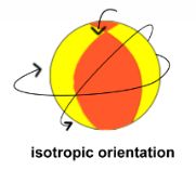
Ideally, these local probes that estimate volume of particles should be performed on isotropic or vertical sections, but this rule is often broken. If you perform one of these probes on preferentially-oriented sections, the results will not be unbiased, but you can still get something out of this data. Plot the estimated areas in a histogram and report that these are biased estimates in that the orientation of the particles is not random. In other words, you tried to keep the sectioning in the same orientation for each animal (e.g., coronal), and you realize that over- or under-estimation of the real volumes may occur due to the fact that every orientation in space is not a possibility for the particles. Of course if you use isotropic or vertical sectioning, you won’t have to worry about this bias.
Three probes that estimate particle volume and are suitable for use with number weighted sampling are Nucleator (Gundersen, etal., 1988), Planar Rotator (Vedel Jensen and Gundersen, 1993), and Optical Rotator (Tandrup, etal., 1997). For estimating particle volume, these local probes are thought to be better than the global probe Cavalieri/point-counting because the latter tends to over-estimate (Tandrup, etal., 1997, Fig. 9). For the nucleator, planar rotator, and optical rotator, ‘The overall impression is that the estimation methods give very similar results’ (Tandrup, etal., 1997, p 114, second full paragraph, third sentence). The standard error of the mean divided by the mean values are lower for the optical rotator (Tandrup, etal., 1997, Fig. 10), but this three dimensional estimator is not as fast to use as the two-dimensional probes, the nucleator and the planar rotator. ‘The optical rotator is chosen if very precise estimates on single cells are necessary’ (Evans, etal., 2004. Chapter 9, Introduction, p 198, last sentence).
Nucleator


Planar Rotator
The planar rotator (Vedel Jensen and Gundersen, 1993) comes in two forms, Isotropic Planar Rotator or Vertical Planar Rotator, depending on if isotropic or vertical sections are used. Computer simulations show the variance of the estimates is lower than with the nucleator (Vedel Jensen and Gundersen, 1993, Fig. 5). This probe is based on the Pappus-Guldinus theorum (Vedel Jensen and Gundersen, 1993, section 3): “If any planar figure revolves about an external axis in its plane, the volume of the solid so generated is equal to the product of the area of the figure and the distance travelled by the center of gravity of the figure”.
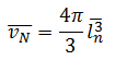
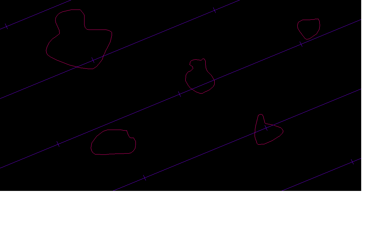
For the vertical planar rotator, pick the particles without bias using a disector for number weighted sampling on vertical sections. The vertical axis is drawn through a point in the particle cross-section, usually the nucleolus. It is fine to use one point to decide if the cell is in the study (see Criteria for Counting Cells) and another point, such as the nucleolus, to be on the vertical axis. Now you indicate the highest and lowest point through the cell profile, and this defines ‘h’. A grid of lines is randomly positioned parallel to ‘h’, and you define the spacing, ‘t’, among these lines.
The event that is marked is the intersection of the lines with the boundary of the particle (red x’s). Then for each line, the distance from the vertical to the ‘red x’ is calculated in both directions (+ direction is to the right and – direction is to the left), and both distances are squared, and the mean of the two squared values is calculated (Vedel Jensen and Gundersen, 1993, table 1 and figure 6), this value is called ‘li2‘. If there are two intersections in a given direction both intersections are marked; in other words if the line at first does not go through the cross section but then encounters it (Vedel Jensen and Gundersen, Fig. 6, see the i=3 line) both distances are squared, the resulting squares are subtracted and divided by two to represent only the part of the cross section the line goes through (see line-row i=3 and columns li,1- and li,2- in Vedel Jensen and Gundersen, 1993, table 1). To calculate the volume estimate:
V = π (t) ∑ li2 (Vedel Jensen and Gundersen, 1993, table 1)
V = volume estimate
t = distance between parallel lines
li2 = [(distance from the vertical to the red x on the right)2 + (distance from the vertical to the red x on the left)2] / 2
For the isotropic planar rotator you can pick the axis you want, so make it along the long axis of the particle. Like the vertical planar rotator, the axis needs to go through a point in the cross-section, usually a nucleolus, and the top and bottom of the cross section are marked to define ‘h’, and then parallel lines perpendicular to ‘h’ with a spacing of ‘t’ are superimposed. But another term is needed, the distance from the nucleolus or point to each parallel line is called ‘ai‘. Also a function called gi(l) and three terms, gi+, gi-, and gi must be defined:

gi+, = gi(l) for directions from the axis to the right, j odd is subtracted from j even so that only the part of the line in the cross section is used
gi+, = gi(l) for directions from the axis to the left
ai = distance from the nucleolus or unique point to the parallel lines
l = distance from axis to boundary
The volume estimate is calculated like this:
V = 2 (t) ∑ gi (Vedel Jensen and Gundersen, 1993, table 2)
V = volume estimate
t = distance between parallel lines
l = distance from axis to boundary
Discrete Vertical Rotator
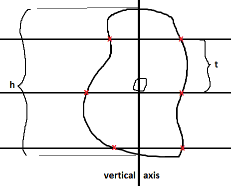
The discrete vertical rotator (Mironov and Mironov, 1997) is a variant of the vertical planar rotator. It was designed to estimate the volume of sub-cellular organelles, such as mitochondria or golgi apparatus, as viewed in ultra-thin electron micrographs. However, instead of marking intersects, the volume is estimated with discrete packets of points (green triangles below). The Pappus-Guldinus theorum states that if a plane is rotated about its edge in space to create a three-dimensional object, the volume of that object will be the product of the area of the plane and the distance that the centroid of the plane has traveled during its rotation. A unique point inside of the cell is used, and that unique point is the centriole (shown in red in the figure below). This is what makes this probe uniquely suited to electron micrographs; the centriole does double duty as both the point used for sampling (the discrete vertical rotator gives a number weighted volume estimate) and for the probing itself. The vertical direction must be indicated in the StereoInvestigator software. Then the main vertical line is set down through the centriole, and parallel lines are also drawn to indicate distance zones. Your job is to mark all of the points that fall on the organelle whose aggregate volume we are estimating (green triangles):
illustration is after Mironov and Mironov, 1997, Fig. 3
est v = π / n (ap) ∑ Pi Di
est v = estimated volume of all the organelles together (the cross sections are shown in blue hash-marks above)
n = number of centriolar sections (one is shown above)
ap = area per point (white plus signs)
Pi = number of points per distance group
Di = distance from center vertical line to distance group
The area is the number of points times the area associated with each point; the distance traveled by the centroid of the area is π times Di. Note that every point within a given distance group (the distance groups are denoted by the white parallel lines above) is considered to have the same Di. In the example above:
ap =1,039 square microns
Pi for distance group one = 5
Di for distance group one = 125 microns
Pi for distance group two = 2
Di for distance group two = 250 microns
For this example:
est v = π / n (ap) ∑ Pi Di
= 22/7 (1,039 square microns) [(5 * 125 microns) + (2 * 250 microns)]
= 367 x 104 cubic microns
The farther away the organelles are from the vertical center line (through the centriole) the greater is the volume attributed to those organelles, because there is more volume farther away from then closer to the vertical line: in other words if the area is rotated around, the centroid of the area travels a farther distance.
“The discretized rotator gave practically identical results to the classic rotator, which is more efficient than the nucleator” (Mironov and Mironov, pg 33, end of second paragraph and also see Table 1).
Optical Rotator
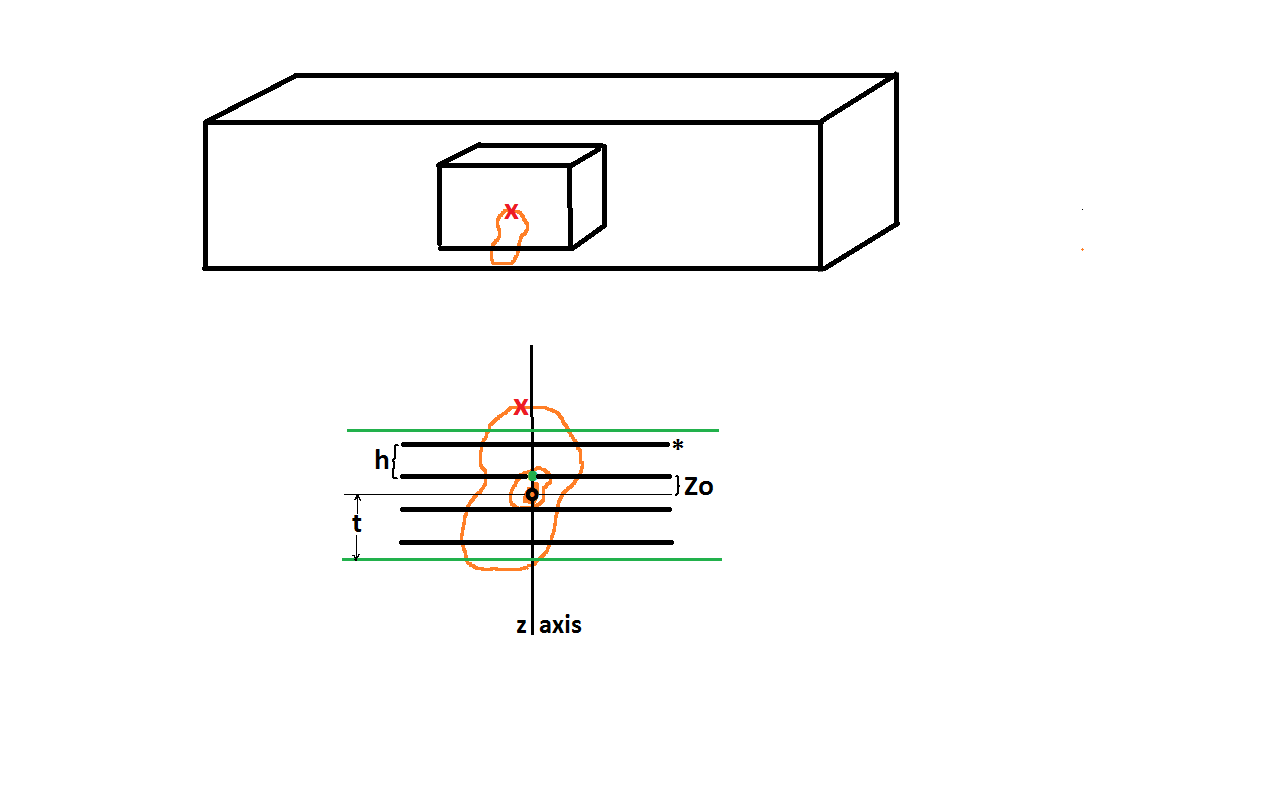
The optical rotator (Tandrup, etal., 1997), unlike the Planar Rotator and Nucleator (see above), uses information from three dimensions for the volume estimate. An optical disector is used to pick cells without bias so that thick sections are being used (see top of figure below) allowing for particle cross sections at different z-planes to be observed. As usual, use sytematic random sampling. If you don’t use systematic random sampling or random sampling to pick the particles for volume estimation, you will not be getting a good idea of what is going on throughout the whole region; and systematic random sampling is more efficient than random sampling.
As for the nucleator and the planar rotator, pick a unique point in the middle of the cell (Tandrup, etal., 1997, see ‘O’ in fig. 2 and see the ‘o’ in the bottom of the figure below), and this point may be different than the point you used to include the cell in the disector (see the red ‘x’ in the figure below). For instance you can use the top of the cell (red ‘x’) to decide if the particle is in the disector, and focus down to a nucleolus (black ‘o’) for this local optical rotator probe. A virtual slice of known thickness (Tandrup, etal., 1997, see ‘t’ in fig. 1, and also see ‘t’ in the bottom of the figure below) with its midpoint (thin black line going through ‘o’ below) through the unique point is generated; in the figure below this thickness, 2t, is bordered by the green lines. The thickness of the virtual slice could be the minimum cell diameter or the mean cell diameter (Tandrup, etal., 1997, fig. 6), as long as the ambiguous top and bottom of the particle are not included. Now the three dimensional part comes in. A distance of random length but less than ‘t’ from the unique point in the middle of the cell along the focusing axis is generated (Tandrup, etal., 1997, see ‘zo‘ in fig. 1). In the bottom of the figure below this is Zo, the distance from the unique point, o, to the green dot. Systematic random optical planes are designated starting there with a distance of ‘h’ separating them (Tandrup, etal., 1997, fig. 1).
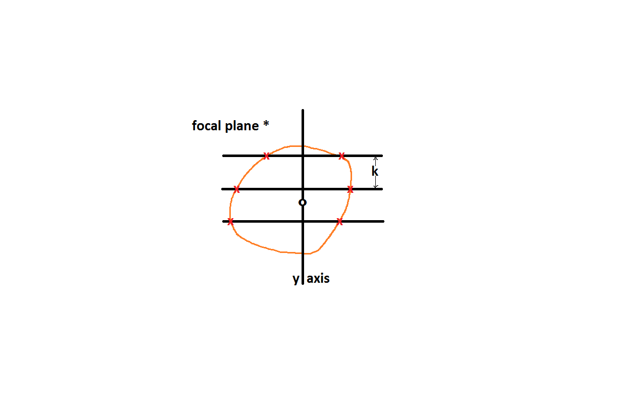
As you focus to each optical plane (four thick black lines within the green lines above) you will see parallel lines forming a grid. One of these planes is shown in the figure below; the asterisk shows this is one focal plane from the figure above. At each plane you mark where the lines of the grid intersect the boundary of the cross section of the particle (Tandrup, etal., 1997, fig. 3 and fig. 6 and see red ‘x’s’ below). The parallel lines emanate from an axis (y-axis, below) that is in the same relative place as the nucleolus (black ‘o’above is on the nucleolus, black ‘o’below is lined up with that, see Tandrup, etal., 1997, open circles and nucleolus in figure 6). For each focal plane the lines are ninety degrees offset from each other; in the next focal plane the probing lines will be oriented up and down instead of horizontally as below. To account for particle cross sections with concavities, those stretches of the line that go through the cross section are given a positive sign and those that traverse the outside of the cross section get negative signs (Tandrup, etal., 1997, fig. 3).
For the isotropic optical rotator isotropic sections are used, and any grid orientation may be used for the first optical plane, and on subsequent planes the orientation of the grid will alternate between perpendicular and parallel to this first orientation (Tandrup, etal., 1997, fig. 6, last sentence in figure legend). The volume estimate is calculated like so:
v = a Σ g(Pi) (Tandrup, etal., 1997, equation 1)
v = volume estimate
a = h * k (Tandrup, etal., 1997, Fig. 2, figure legend and also see figures above: h is the distance between focal planes and k is the distance between parallel lines on a given focal plane, so a is the density of intersecting lines)
g(P) varies (Tandrup, etal., 1997, equation 2):
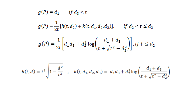
To understand these equations please refer to figure 2 in Tandrup, etal., 1997.
g(P) is a function dependent on where the intercept, P is located (red x’s in figure above)
d1, d2, and d3 are one, two, and three dimensional distances, respectively
d1 = the distance from Pi to the projection of the unique point ‘o’ along the z-axis to the plane that Pi is in
d2 = the shortest distance from the grid line on the cross section to the unique point ‘o’
d3= the distance from Pi to the unique point ‘o’
t = one half of the thickness of optical slice, distance from unique point ‘o’ to green line in top figure
For the vertical optical rotator, vertical sections are used (Tandrup, etal., 1997, Fig. 5) and the vertical axis is the vertical line that the parallel lines originate from on the cross section. In other words, in the figure above, the line labeled ‘y-axis’ is the vertical axis. The line orientation alternates by ninety degrees for each focal plane. Other than keeping track of the vertical axis, the marking of events is the same as for the isotropic optical rotator (red x’s in figure above). The volume is calculated with the same formula:
v = a Σ g(P) (Tandrup, etal., 1997, equation 1)
v = volume estimate
a = h * k (see figures above, h is the distance between focal planes and k is the distance between parallel lines on a given focal plane, so a is the density of intersecting lines)
but g(P) varies differently than for the isotropic vertical rotator, including the addition of the term ‘z’. Also, unlike the isotropic optical rotator, there are separate formulas for g as a function of P depending on whether the lines are parallel or perpendicular to the vertical axis. For lines parallel to the vertical axis (Tandrup, etal., 1997, equations 4):

but for lines perpendicular to the vertical axis (Tandrup, etal., 1997, equations 5):
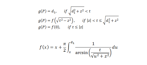
z = the distance from the plane containing the unique point ‘o’ to the given optical plane (called Zo in the figures above)
The integrals regarding f as a function of x above “have no analytical solution, but can be solved numerically, e.g., by adjusted Simpson integration” (Tandrup, etal., 1997, p. 6, text below equations 5b and 5c).
Point-Sampled-Intercepts
When using point-sampled-intercepts (Sorenson, 1991) sampling to obtain a volume-weighted estimate of volume, you could use the nucleator probe (see directly above) to make the individial estimates, but:
“Since the point is random inside the particle, it is not efficient to make two measurements in two opposite directions from the point, it is better to measure the length of the complete intercept through the point in a 3-dimensionally isotropic direction (on IUR or “vertical” sections). The coefficient to be used for calculating the volume-weighted mean particle volume, V v , is then π/3 instead of 4π/3. This special case of the general nucleator principle was described before the nucleator and has its own name, point-sampled linear intercepts, which also describes reasonably precisely what it involves.” (Gundersen etal., 1988, pg. 163, bottom of last complete paragraph).
In other words, we already have an intercept through a cross section of the particle, so why not use it to estimate volume? In the example below, two particle-cross-sections are selected (it is more likely for larger particles to be selected, that is why it is called a volume weighted estimate of volume):
this one:

and this one:

The distance between the two red triangles is cubed and multiplied by π/3 to estimate the mean volume weighted volume (Sorensen, 1991, equation 2 and Evans, 2004, equation 5.1):
Vv = π/3 (l3) [if there is more than one intercept through the cross section of a particle, take the mean of the cubed intercept length]
Vv = volume weighted estimate of volume
l = intercept length
The intercept length, collected in a volume-weighted way is of interest when characterizing alveoli in lung (Knudsen, etal., 2010). Intercepts have also been used to estimate particle volume when the particles have been selected in a number weighted manner, i.e. by using a disector (Cruz-Orize, 1987).
Surface Weighted Star Volume
The concept of star volume (Vesterby, 1993) helps to study cells and lacunae, holes and spaces that are complex. “The star volume of an object is defined as the mean size of the object when seen unobscured along uninterrupted straight lines in all possible directions from random points inside the object” (Vesterby, 1993, p. 327, STAR VOLUME OF MARROW SPACE). If an object is convex, its star volume is the same as its volume. If there is a concavity, the star volume is less than the volume (Reed and Howard, 1998, Fig. 1). For the surface weighted star volume probe, you can use the Gittes method (Reed and Howard, 1998, section 2.3) of sampling, that is a form of surface weighted sampling. Only isotropic sections can be used. The intercepts drawn across the volume from the surface (Reed and Howard, 1998, Fig. 2) can be used to calculate the surface weighted star volume:
Vs = 2/3 π l3 (Reed and Howard, 1998, equation 2)
Vs = surface weighted volume estimate
l = mean intercept length
Cruz-Orize, LM. (1987) Particle Number can be Estimated Using a Disector of Unknown Thickness: the Selector, J. of Microscopy, 145 121 – 142.
Evans, S.M., A.M. Janson, J.R. Nyengaard, 2004 Quantitative Methods in Neuroscience, Oxford University Press, Oxford, U.K.
Knudsen, L., Weibel, E.R., Gundersen, H.J.G., Weinstein, F.V., and M. Ochs (2010) Assessment of Air Space Size Characteristics by Intercept (Chord) Measurement: an Accurate and Efficient Stereological Approach. J. of Applied Physiology, 108, 412 – 421.
Gundersen, H.J.G., and R. Osterby, 1981, Optimizing Sampling Efficiency of Stereological Studies in Biology: or ‘Do more less well!’. J. of Microscopy, Vol. 121, pp. 65-73.
Gundersen, H.J.G., 1988, The Nucleator. J. of Microscopy, Vol. 151, pp. 3-21.
Gundersen, H.J.G., Bagger, P., Bendtsen, T.F., Evans, S.M., Korbo, L., Marcussen, N., Moller, A., Nielsen, K., Nyengaard, J.R., Pakkenberg, B., Sorensen, F.B., Vesterby A., and M.J. West (1988) The New Stereological Tools: Disector, Fractionator, Nucleator and Point Sampled Intercepts and their Use in Pathological Research and Diagnosis, APMIS, 96, 857 – 881.
Howard, C.V. and M.G. Reed, 2011, Unbiased Stereology, Second Edition QTP Publications, Liverpool, U.K.
Mironov, A.A. Jr. and A.A. Mironov (1997) Estimation of Subcellular Organelle Volume from Ultrathin Sections through Centrioles with a Discretized Version of the Vertical Rotator, J. of Microscopy, 192, 29 – 36.
Reed, M.G. and C.V. Howard (1998) Surface-weighted Star Volume: Concept and Estimation, J. of Microscopy, 190, 350 – 356.
Sorensen F.B. (1991) Stereological Estimation of the Mean and Variance of Nuclear Volume from Vertical Sections, J. of Microscopy, 162, 203 – 229.
Tandrup, T., Gundersen, H.J.G. and E.B. Vedel Jensen (1997) The Optical Rotator. J. of Microscopy, 186, 108 -120.
Vedel Jensen, E.B. and H.J.G. Gundersen (1993) The Rotator. J. of Microscopy, 170, 35 – 44.
Vesterby, A. (1993) Star Volume in Bone Research, Anatomical Record, 235, 325 – 334.
